
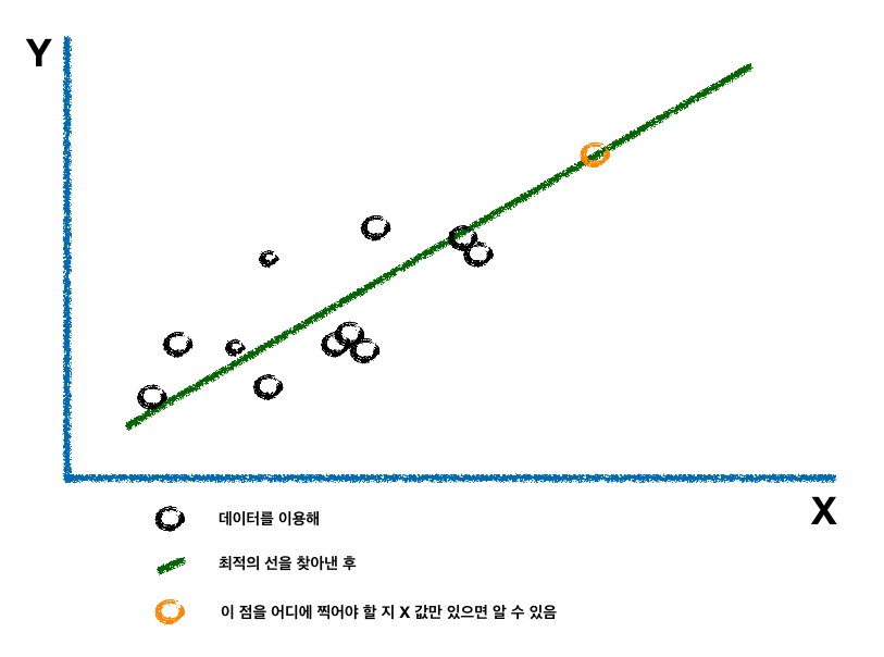
- 주어진 x와 y 값을 가지고 서로 간의 관계를 파악
- 새로운 x값이 주어졌을 때 y값을 쉽게 알 수 있음
In [1]:
import tensorflow as tf
In [2]:
x_data = [1, 2, 3]
y_data = [1, 2, 3]
data 생성
In [3]:
W = tf.Variable(tf.random_uniform([1], -1.0, 1.0))
b = tf.Variable(tf.random_uniform([1], -1.0, 1.0))
placeholder 설정
In [4]:
X = tf.placeholder(tf.float32, name="X")
Y = tf.placeholder(tf.float32, name="Y")
model 설정
In [5]:
model = W*X + b
cost function
In [6]:
cost = tf.reduce_mean(tf.square(model- Y))
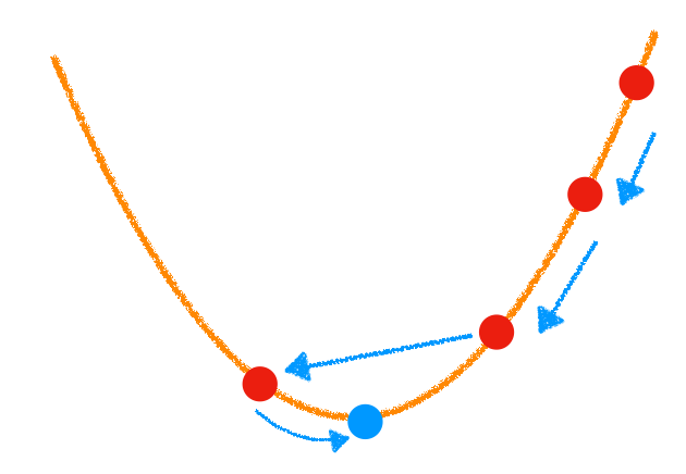
gradient desent
In [7]:
optimizer = tf.train.GradientDescentOptimizer(learning_rate=0.1)
train_op = optimizer.minimize(cost)
modeling
In [8]:
sess =  tf.Session()
sess.run(tf.global_variables_initializer())
for step in range(500):
    _, cost_val = sess.run([train_op, cost], feed_dict={X: x_data, Y: y_data})
    if step % 25 == 0:
        print("step: {}, cost_val: {:.5f}, W: {}, b: {}".format(step, cost_val, sess.run(W), sess.run(b)))
test
In [9]:
class prediction:

    def run(self, input):
        self.input = input
        output = sess.run(model, feed_dict={X: self.input})
        print("X: {}, Y-result: {}".format(self.input, output))

pred = prediction()
In [10]:
pred.run(2.5)
pred.run(5)
pred.run(10)
In [11]:
from IPython.core.display import HTML, display

display(HTML("<style> .container{width:100% !important;}</style>"))
'Deep_Learning' 카테고리의 다른 글
| 06.tensorboard01_example (0) | 2018.12.09 |
|---|---|
| 05.deep_neural_net_Costfun2 (0) | 2018.12.09 |
| 04.deep_neural_net_Costfun1 (0) | 2018.12.09 |
| 03.classification (0) | 2018.12.09 |
| 01.tesnsor_and_graph (0) | 2018.12.09 |