15.RNN_mnist

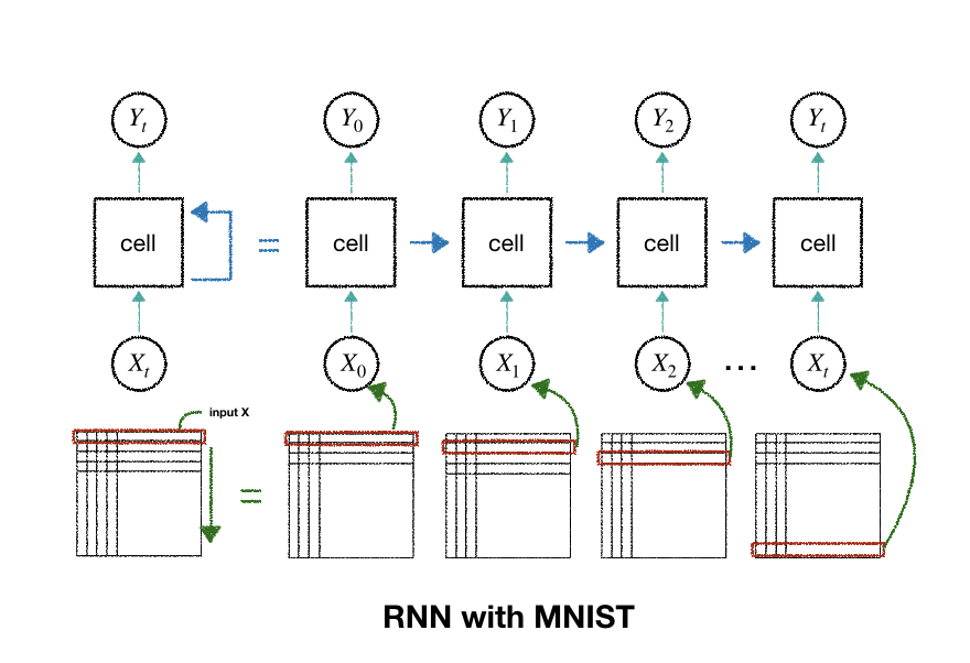
  • 이 그림의 가운데에 있는 한 덩어리의 신경망을 RNN에서는 Cell이라 부름
  • cell을 여러개 중첩하여 심층 신경망을 만듬
  • 앞 단계에서 학습한 결과를 다음 단계의 학습에 이용
  • 따라서 학습 데이터를 단계별로 구분하여 입력

  • 사람은 글씨를 위에서 아래로 내려가면서 쓰는 경향이 많으므로
  • 가로 한줄의 28 픽셀을 한 단계의 입력값으로 삼고
  • 세로줄이 총 28개 이므로 28단계를 거쳐 데이터를 입력 받음


library load

In [1]:
import tensorflow as tf
import numpy as np
In [3]:
from tensorflow.examples.tutorials.mnist import input_data
mnist = input_data.read_data_sets("./mnist/data/", one_hot=True)
Extracting ./mnist/data/train-images-idx3-ubyte.gz
Extracting ./mnist/data/train-labels-idx1-ubyte.gz
Extracting ./mnist/data/t10k-images-idx3-ubyte.gz
Extracting ./mnist/data/t10k-labels-idx1-ubyte.gz


hyper parameter

  • 입력값 X에 n_step이라는 차원을 하나 더 추가
  • RNN은 순서가 있는 데이터를 다루므로 한 번에 입력 받을 갯수와 몇 단계로 이뤄진 데이터를 받을지를 설정
  • 가로 픽셀 수를 n_input, 세로 픽셀 수를 입력 단계인 n_step으로 설정
  • 앞에서 설명한 대로 RNN은 순서가 있는 데이터를 다루므로 한 번에 입력 받을 갯수와 총 몇 단계로 이뤄진 데이터를 받을지를 설정
  • 가로 픽셀수: n_input, 세로 픽셀수: n_step
  • 출력값은 계속해서 온 것처럼 MNIST의 분류인 0~9까지 10개의 숫자를 one-hot encoding으로 표현
In [4]:
learning_rate = 0.001
total_epoch = 30
batch_size = 128

n_input = 28
n_step = 28
n_hidden = 128
n_class = 10

X = tf.placeholder(tf.float32, [None, n_step, n_input], name="input_X")
Y = tf.placeholder(tf.float32, [None, n_class], name="output_Y")
W = tf.Variable(tf.random_normal([n_hidden, n_class], name="weight_W"))
b = tf.Variable(tf.random_normal([n_class], name="bias_b"))


hidden개의 출력값을 갖는 RNN cell을 생성

In [5]:
cell = tf.nn.rnn_cell.BasicRNNCell(n_hidden)
WARNING:tensorflow:From <ipython-input-5-e006f918b220>:1: BasicRNNCell.__init__ (from tensorflow.python.ops.rnn_cell_impl) is deprecated and will be removed in a future version.
Instructions for updating:
This class is equivalent as tf.keras.layers.SimpleRNNCell, and will be replaced by that in Tensorflow 2.0.
  • BasicLSTMCell, GRUCell 등 다양한 방식의 셀을 사용
  • RNN의 기본신경망은 긴 단계의 데이터를 학습할 때 맨 뒤에서는 맨 앞의 정보를 잘 기억하지 못하는 특성이 존재
  • 이를 보완하기 나온 것이 LSTMLong Short-Term Memory, GRUGated Recurrent Units
  • GRU는 LSTM과 비슷하지만, 구조가 조금 더 간단한 신경망 Architecture


complete RNN

In [6]:
outputs, states = tf.nn.dynamic_rnn(cell, X, dtype=tf.float32)


  • 결과값을 one-hot encoding 형태로 만들 것이므로 손실 함수로 tf.nn.softmax_cross_entropy_with_logits_v2를 사용
  • 이 함수를 사용하려면 최종 결과값이 [batch_size, n_class] 여야 함
  • RNN 신경망에서 나오는 출력값은 [batch_size, n_step, n_hidden]
In [7]:
# outputs : [batch_size, n_step, n_hidden]
outputs = tf.transpose(outputs, [1, 0, 2]) # index를 기준으로 transpose
outputs = outputs[-1]


modeling

$y = (X \times W) +b$

In [8]:
model = tf.matmul(outputs, W) + b
cost = tf.reduce_mean(tf.nn.softmax_cross_entropy_with_logits_v2(logits=model, labels=Y))
opt = tf.train.AdamOptimizer(learning_rate=learning_rate).minimize(cost)


variable initializer

In [9]:
init = tf.global_variables_initializer()
sess = tf.Session()
sess.run(init)
In [10]:
x_train = mnist.train.images
y_train = mnist.train.labels
In [11]:
class Dataset:
    def __init__(self, x, y):
        self.index_in_epoch = 0
        self.epoch_completed = 0
        self.x_train = x
        self.y_train = y
        self.num_examples = x.shape[0]
        
    def data(self):
        return self.x_train, self.y_train
    
    def next_batch(self, batch_size):
        start = self.index_in_epoch
        self.batch_size = batch_size
        self.index_in_epoch += self.batch_size
        
        if start==0 and self.epoch_completed==0:
            idx = np.arange(self.num_examples)
            np.random.shuffle(idx)
            self.x_train = self.x_train[idx]
            self.y_train = self.y_train[idx]
            
        if start + batch_size > self.num_examples:            
            self.epoch_completed += 1
            
            perm = np.arange(self.num_examples)
            np.random.shuffle(perm)
            self.x_train = self.x_train[perm]
            self.y_train = self.y_train[perm]

            start = 0
            self.index_in_epoch = self.batch_size

        end = self.index_in_epoch
        return self.x_train[start:end], self.y_train[start:end]
In [12]:
total_batch = int(x_train.shape[0]/batch_size)
epoch_cost_val_list = []
cost_val_list = []
for epoch in range(total_epoch):
    epoch_cost = 0
    for i in range(total_batch):
        batch_xs, batch_ys = Dataset(x=x_train, y=y_train).next_batch(batch_size=batch_size)
        batch_xs = batch_xs.reshape([batch_size, n_step, n_input])
        
        _, cost_val = sess.run([opt, cost], feed_dict={
            X: batch_xs, Y: batch_ys
        })
        
        epoch_cost += cost_val
        cost_val_list.append(cost_val)        
        
    epoch_cost_val_list.append(epoch_cost)   
    
    if (epoch+1) %5 == 0:
        print("Epoch: %04d" % (epoch+1),
              "Avg.cost = {}".format(epoch_cost/total_batch))
    
print("\noptimization complete")

is_correct = tf.equal(tf.argmax(model, 1), tf.argmax(Y, 1))
accuracy = tf.reduce_mean(tf.cast(is_correct, tf.float32))

test_batch_size = len(mnist.test.images)
test_xs = mnist.test.images.reshape(test_batch_size, n_step, n_input)
test_ys = mnist.test.labels

print("\naccuracy {:.3f}%".format(
    sess.run(accuracy*100, feed_dict={X: test_xs, Y: test_ys})
))
Epoch: 0005 Avg.cost = 0.13626715096716696
Epoch: 0010 Avg.cost = 0.0966348738251102
Epoch: 0015 Avg.cost = 0.08380235770244003
Epoch: 0020 Avg.cost = 0.07091071723204861
Epoch: 0025 Avg.cost = 0.07897876071068513
Epoch: 0030 Avg.cost = 0.05630091918466313

optimization complete

accuracy 97.660%
In [14]:
import matplotlib.pyplot as plt

plt.rcParams["axes.unicode_minus"] = False

_, ax = plt.subplots(1, 2, figsize=(20, 5))
ax[0].set_title("cost_epoch")
ax[0].plot(epoch_cost_val_list, linewidth=0.3)
ax[1].set_title("cost_value")
ax[1].plot(cost_val_list, linewidth=0.3)
plt.show()
In [16]:
from IPython.core.display import HTML, display

display(HTML("<style> .container{width:100% !important;}</style>"))

'Deep_Learning' 카테고리의 다른 글

17.seq2seq  (0) 2018.12.19
16.RNN_word_autoComplete  (0) 2018.12.18
14.gan  (0) 2018.12.16
13.auto-encoder  (0) 2018.12.15
12.mnist_cnn  (0) 2018.12.12
11.mnist_matplotlib
In [1]:
import pandas as pd
import numpy as np
import tensorflow as tf
import matplotlib.pyplot as plt

plt.rcParams["axes.unicode_minus"] = False
plt.rcParams["figure.figsize"] = (12, 8)
In [3]:
from tensorflow.examples.tutorials.mnist import input_data
mnist = input_data.read_data_sets("./mnist/data/", one_hot=True)
Extracting ./mnist/data/train-images-idx3-ubyte.gz
Extracting ./mnist/data/train-labels-idx1-ubyte.gz
Extracting ./mnist/data/t10k-images-idx3-ubyte.gz
Extracting ./mnist/data/t10k-labels-idx1-ubyte.gz


variable setting

In [4]:
global_step = tf.Variable(0, trainable=False, name="global_step")
X = tf.placeholder(tf.float32, shape=[None, 784], name="X")
Y = tf.placeholder(tf.float32, shape=[None,  10], name="Y")

W1 = tf.Variable(tf.random_normal([784, 256], mean=0, stddev=0.01), name="W1")
W2 = tf.Variable(tf.random_normal([256, 256], mean=0, stddev=0.01), name="W2")
W3 = tf.Variable(tf.random_normal([256,  10], mean=0, stddev=0.01), name="W3")

b1 = tf.zeros([256], name="bias1")
b2 = tf.zeros([256], name="bias2")
b3 = tf.zeros([10] , name="bais3")


model setting

In [5]:
keep_prob = tf.placeholder(tf.float32)

with tf.name_scope("layer1"):
    L1 = tf.add(tf.matmul(X, W1), b1)
    L1 = tf.nn.relu(L1)
    L1 = tf.nn.dropout(L1, keep_prob)
    
with tf.name_scope("layer2"):
    L2 = tf.add(tf.matmul(L1, W2), b2)
    L2 = tf.nn.relu(L2)
    L2 = tf.nn.dropout(L2, keep_prob)
    
with tf.name_scope("layer3"):
    model = tf.add(tf.matmul(L2, W3), b3)
    
with tf.name_scope("cost"):
    cost = tf.reduce_mean(
        tf.nn.softmax_cross_entropy_with_logits_v2(labels=Y, logits=model))
    opt = tf.train.AdamOptimizer(0.001).minimize(cost, global_step=global_step)
    
    tf.summary.scalar("cost", cost)


model initialization

In [6]:
init = tf.global_variables_initializer()
sess = tf.Session()

sess.run(init)

merged = tf.summary.merge_all()
writer = tf.summary.FileWriter("./logs/mnist_matplotlib", sess.graph)
In [7]:
batch_size = 50
total_batch = int(mnist.train.num_examples / batch_size)
cost_epoch = []


model training

In [8]:
%%time
for epoch in range(20):
    total_cost = 0
    
    for i in range(total_batch):
        batch_xs, batch_ys = mnist.train.next_batch(batch_size)
        
        _, cost_val = sess.run([opt, cost], feed_dict={X:batch_xs, Y: batch_ys, keep_prob:0.8})
        total_cost += cost_val
        cost_epoch.append(total_cost)
        
        summary = sess.run(merged, feed_dict={X:batch_xs, Y: batch_ys, keep_prob:0.8})
        writer.add_summary(summary, global_step=sess.run(global_step))
        
    print("epoch: %d, Avg.cost: %.4f" % (
        epoch+1, total_cost / total_batch
    ))
epoch: 1, Avg.cost: 0.3481
epoch: 2, Avg.cost: 0.1395
epoch: 3, Avg.cost: 0.1000
epoch: 4, Avg.cost: 0.0806
epoch: 5, Avg.cost: 0.0697
epoch: 6, Avg.cost: 0.0591
epoch: 7, Avg.cost: 0.0507
epoch: 8, Avg.cost: 0.0455
epoch: 9, Avg.cost: 0.0417
epoch: 10, Avg.cost: 0.0394
epoch: 11, Avg.cost: 0.0362
epoch: 12, Avg.cost: 0.0361
epoch: 13, Avg.cost: 0.0305
epoch: 14, Avg.cost: 0.0303
epoch: 15, Avg.cost: 0.0271
epoch: 16, Avg.cost: 0.0282
epoch: 17, Avg.cost: 0.0267
epoch: 18, Avg.cost: 0.0267
epoch: 19, Avg.cost: 0.0219
epoch: 20, Avg.cost: 0.0238
CPU times: user 3min 22s, sys: 43.7 s, total: 4min 6s
Wall time: 2min 27s


cost function

In [9]:
plt.figure(figsize=(20, 8))
plt.plot(cost_epoch, "g")
plt.title("cost_epoch")
plt.show()


tensor graph

In [10]:
## jptensor.py 를 워킹디렉토리에 import
import jptensor as jp

tf_graph = tf.get_default_graph().as_graph_def()
jp.show_graph(tf_graph)


test

In [11]:
is_correct = tf.equal(tf.argmax(model, 1), tf.argmax(Y, 1))
accuracy = tf.reduce_mean(tf.cast(is_correct, tf.float32))

accuracy_val = sess.run(accuracy, feed_dict={X: mnist.test.images, 
                                             Y: mnist.test.labels,
                                             keep_prob: 1})

print("accuracy: %.3f" % (accuracy_val))
accuracy: 0.980


labels

In [12]:
labels = sess.run(model, feed_dict={X: mnist.test.images,
                                    Y: mnist.test.labels,
                                    keep_prob: 1})
In [13]:
%matplotlib inline
fig = plt.figure()
for i in range(10):
    # (2, 5)의 그래프, i + 1번째 숫자 이미지 출력
    subplot = fig.add_subplot(2, 5, i+1)
    
    # x, y축 눈금 제거
    subplot.set_xticks([])
    subplot.set_yticks([])
    
    # 출력한 이미지 위에 예측한 숫자를 출력
    # np.argmax와 tf.argmax는 같은 기능
    # 결과값인 labels의 i번째 요소가 one-hot encoding으로 되어 있으므로
    # 해당 배열에서 가장 높은 값을 가진 인덱스를 예측한 숫자로 출력
    subplot.set_title("%d" % (np.argmax(labels[i])))
    
    # 1차원 배열로 되어 있는 i번째 이미지 데이터를
    # 28 x 28형태의 2차원 배열로 변환
    subplot.imshow(mnist.test.images[i].reshape((28, 28)))
plt.show()
In [14]:
from IPython.core.display import HTML, display

display(HTML("<style> .container{width:100% !important;}</style>"))

'Deep_Learning' 카테고리의 다른 글

13.auto-encoder  (0) 2018.12.15
12.mnist_cnn  (0) 2018.12.12
10.mnist_dropout  (0) 2018.12.10
00.write_csv  (0) 2018.12.09
09.mnist_01_minibatch  (0) 2018.12.09

+ Recent posts